Data Analysis in a Natural Selection Simulation
I really like the HHMI Biointeractive activity “Battling Beetles”. I have used it, in some iteration (see below), for the last 6 years to model certain aspects of natural selection. There is an extension where you can explore genetic drift and Hardy-Weinberg equilibrium calculations, though I have never done that with my 9th graders. If you stop at that point, the lab is lacking a bit in quantitative analysis. Students calculate phenotypic frequencies, but there is so much more you can do. I used the lab to introduce the idea of a null hypothesis and standard error to my students this year, and I may never go back!
We set up our lab notebooks with a title, purpose/objective statements, and a data table. I provided students with an initial hypothesis (the null hypothesis), and ask them to generate an alternate hypothesis to mine (alternative hypothesis). I didn’t initially use the terms ‘null’ and ‘alternative’ for the hypotheses because, honestly, it wouldn’t have an impact on their success, and those are vocabulary words we can visit after demonstrating the main focus of the lesson. When you’re 14, and you’re trying to remember information from 6 other classes, even simple jargon can bog things down. I had students take a random sample of 10 “male beetles” of each shell color, we smashed them together according the HHMI procedure, and students reported the surviving frequencies to me.
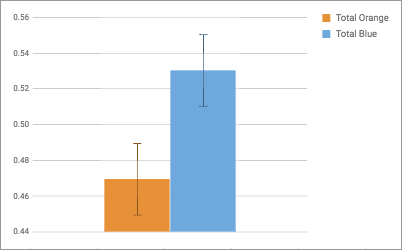
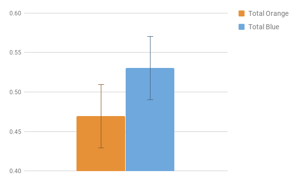
Once I had the sample frequencies, I used a Google Sheet to find averages and standard error, and reported those to my students. Having earlier emphasized “good” science as falsifiable, tentative and fallible, we began to talk about “confidence” and “significance” in research. What really seemed to work was this analogy: if your parents give you a curfew of 10:30 and you get home at 10:31, were you home on time? It isn’t a perfect comparison, and it is definitely something I’ll regret when my daughter is a few years older, but that seemed to click for most students. 10:31 isn’t 10:30, but if we’re being honest with each other, there isn’t a real difference between the two. After all, most people would unconsciously round 10:31 down to 10:30 without thinking. We calculated the average frequency changed from 0.5 for blue M&M’s to 0.53, and orange conversely moved from 0.5 to 0.47. So I asked them again: Does blue have an advantage? Is our result significant?
Short story, no; we failed to reject the null hypothesis. Unless you are using a 70% confidence interval, our result is not significantly different based on 36 samples. But it was neat to see the interval shrink during the day. After each class period, we added a few more samples, and the standard error measurement moved from 0.05 to 0.03 to 0.02. It was a really powerful way to emphasize the importance of sample size in scientific endeavors.
Should the pattern (cross-cutting concept!) hold across 20 more samples, the intervals would no longer overlap, and we could start to see something interesting. So if anyone has a giant bag of M&M’s lying around and you want to contribute to our data set, copy this sheet, add your results, and share it back my way. Hope we can collaborate!
Email results, comments, questions to Drew Ising at aising@usd348.com or drewising@gmail.com
–Versions of Battling Beetles Lab I’ve Tried–


 Next Post